Getting started with RepLikCompare
This tutorial walks through the main features of RepLikCompare on a worked example: loading a dataset, comparing systems and replicas, clustering conformations, reducing dimensionality, and plotting the results.
The dataset used here (df.csv) is synthetic — it was generated purely to illustrate the package’s workflow and does not come from a real molecular dynamics simulation. It mimics a typical replica-based MD setup: several systems (WT, Mutant_A, Ligand_A, Ligand_B, Flexible), each run as several replicas, with one row per trajectory frame and a handful of numeric collective variables/features commonly seen in MD analysis:
Column |
Description |
|---|---|
|
System/condition (e.g. |
|
Replica index within a system ( |
|
Frame index along the trajectory |
|
Radius of gyration |
|
Solvent-accessible surface area |
|
Root-mean-square deviation |
|
Root-mean-square fluctuation |
|
Number of hydrogen bonds |
|
Potential energy |
|
A circular (angular) collective variable |
We will use these columns as feature/observable examples throughout the tutorial to show what each part of RepLikCompare can do.
[1]:
import RepLikCompare as rlc
import pandas as pd
import matplotlib.pyplot as plt
from IPython.display import display
/usr/local/lib/python3.12/dist-packages/tqdm/auto.py:21: TqdmWarning: IProgress not found. Please update jupyter and ipywidgets. See https://ipywidgets.readthedocs.io/en/stable/user_install.html
  from .autonotebook import tqdm as notebook_tqdm
1. Loading the dataset
RepLikCompare’s Dataset wraps a pandas DataFrame together with simulation/replica metadata. The input table must contain, at minimum, two columns identifying the system and the replica each row belongs to — here sim_name and replica, which Dataset detects automatically.
[2]:
df = pd.read_csv("df.csv", index_col=0)
df.head()
[2]:
| sim_name | replica | frame | cluster_state | Radius_Gyration | SASA | RMSD | RMSF | HBonds | Potential_Energy | Dihedral_Angle | |
|---|---|---|---|---|---|---|---|---|---|---|---|
| 0 | WT | 1 | 0 | 0 | 18.120029 | 162.326932 | 1.584457 | 0.662354 | 205.009943 | -1373.041538 | -96.400189 |
| 1 | WT | 1 | 1 | 0 | 18.349881 | 156.711960 | 1.872718 | 0.773739 | 202.541489 | -1383.147669 | -51.348810 |
| 2 | WT | 1 | 2 | 0 | 19.272076 | 176.338459 | 2.095835 | 0.833684 | 206.182798 | -1369.002222 | -74.037508 |
| 3 | WT | 1 | 3 | 0 | 18.911540 | 159.142525 | 1.671309 | 0.713268 | 207.590998 | -1404.957461 | -86.691822 |
| 4 | WT | 1 | 4 | 0 | 17.879963 | 152.160358 | 1.597107 | 0.730884 | 207.234531 | -1385.006682 | -73.193045 |
[3]:
# A Dataset can be built from an existing DataFrame...
dataset = rlc.Dataset.from_dataframe(df)

# ...or loaded directly from a CSV file (equivalent to the two lines above):
# dataset = rlc.Dataset.from_csv("df.csv", index_col=0)
INFO - Dataset: auto-detected sim_name_col='sim_name'
INFO - Dataset: auto-detected replica_col='replica'
INFO - Dataset: replica_col='replica' has values that repeat across systems (e.g. replica numbers reused per system) -- grouping by it alone would silently merge different systems' replicas in tools that need global uniqueness (compute_jsd, compute_wasserstein). Auto-created column 'System' (= sim_name + '_rep' + replica) and will use it for those tools. `replica_col` itself is left unchanged for filtering (_select_data) and for plot_cluster_timeline.
[4]:
print("sim_name_col:", dataset.sim_name_col)
print("replica_col:", dataset.replica_col)
print("unique_replica_col:", dataset.unique_replica_col)
dataset.df.head()
sim_name_col: sim_name
replica_col: replica
unique_replica_col: System
[4]:
| sim_name | replica | frame | cluster_state | Radius_Gyration | SASA | RMSD | RMSF | HBonds | Potential_Energy | Dihedral_Angle | System | |
|---|---|---|---|---|---|---|---|---|---|---|---|---|
| 0 | WT | 1 | 0 | 0 | 18.120029 | 162.326932 | 1.584457 | 0.662354 | 205.009943 | -1373.041538 | -96.400189 | WT_rep1 |
| 1 | WT | 1 | 1 | 0 | 18.349881 | 156.711960 | 1.872718 | 0.773739 | 202.541489 | -1383.147669 | -51.348810 | WT_rep1 |
| 2 | WT | 1 | 2 | 0 | 19.272076 | 176.338459 | 2.095835 | 0.833684 | 206.182798 | -1369.002222 | -74.037508 | WT_rep1 |
| 3 | WT | 1 | 3 | 0 | 18.911540 | 159.142525 | 1.671309 | 0.713268 | 207.590998 | -1404.957461 | -86.691822 | WT_rep1 |
| 4 | WT | 1 | 4 | 0 | 17.879963 | 152.160358 | 1.597107 | 0.730884 | 207.234531 | -1385.006682 | -73.193045 | WT_rep1 |
A note on naming your replica column. In this dataset,
replicais just1, 2, 3, 4and is reused identically across every system (WT,Mutant_A, … each have their own replica1). That’s fine, but it means the rawreplicacolumn is not a unique trajectory identifier on its own —replica=1alone doesn’t say which system’s replica 1.
Datasetdetects this automatically: since it sawreplicavalues collide across systems, it auto-built a collision-safe column (shown above asunique_replica_col, here namedSystem, built assim_name + "_rep" + replica) and uses it internally wherever a globally-unique trajectory id is required (compute_jsd,compute_wasserstein, andgroup_by="both"incompute_convergence– see below).This auto-detection is a safety net, not a reason to skip thinking about it yourself. If you’re building your own dataset, the more robust convention is to make the replica column unique up front – e.g. name replicas
WT_1,WT_2,Mutant_A_1, … instead of bare1,2,3. Whichever convention you use, always check ``dataset.unique_replica_col`` after creating aDatasetto confirm RepLikCompare resolved it the way you expect.
2. Ensemble comparison
These tools statistically compare the distribution of a feature across systems and/or replicas, to check whether two conditions actually sample different states (and whether replicas of the same system agree with each other, as a baseline).
2.1 Jensen-Shannon divergence — compute_jsd
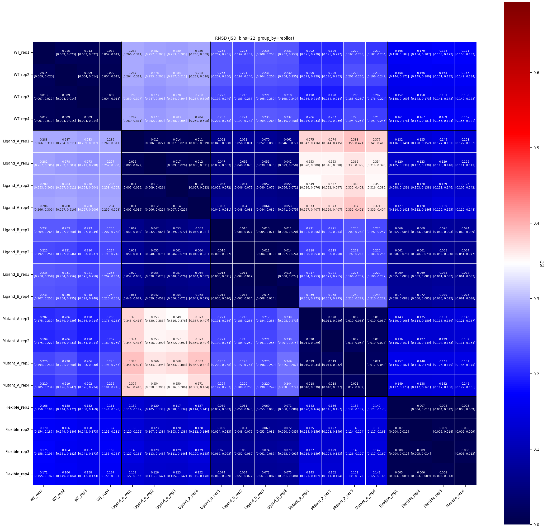
The Jensen-Shannon divergence (bounded in [0, ln(2)] ≈ [0, 0.693]) between distributions, computed with bootstrap resampling and confidence intervals.
Main options:
feature_col: a column name (1D JSD) or a tuple of two columns (2D joint JSD).group_by:"replica"(default — rigorous, compares intra- vs. inter-replica spread) or"system"(pooled — merges all replicas of a system together).is_angle/angle_unit: circular treatment (fixed[-pi, pi]range), with auto-detection of degrees/radians or a forced unit ("deg"/"rad").bins:"auto"/"sqrt"/"sturges"/ an integer, or(bins_x, bins_y)in 2D.iters,frac,replace,seed: bootstrap parameters.confidence_level: confidence-interval level (default0.95).plot_heatmap: draw the summary heatmap (stored intables["heatmap_ax"]).explain: ifTrue(default), also prints a human-readable interpretation (DISTINGUISHABLE/NOT distinguishable/AMBIGUOUS).
Returns: a dict with system_summary, replica_pairs, replica_outliers, system_overall, heatmap_ax, bins_used, and __description__.
[5]:
jsd_rmsd = dataset.compute_jsd(feature_col="RMSD", plot_heatmap=True)
jsd_rmsd["system_summary"][["system_1", "system_2", "inter_mean", "verdict", "effect_magnitude"]]
INFO - === RMSD (RMSD) | metric=jsd | group_by=replica ===
INFO - bins: 'auto' -> 22
bootstrap JSD RMSD: 100%|██████████| 210/210 [00:04<00:00, 45.43pair/s]
============================================================
                RMSD -- quick interpretation
============================================================
(bins used: 22)

+----------------------+-------------------------+----------------------+-----------------+
| System pair          | Inter JSD [95% CI]      | Magnitude (% of ln2) | Verdict         |
+----------------------+-------------------------+----------------------+-----------------+
| WT vs Ligand_A       | 0.2825 [0.2554, 0.3084] | large (40.8%)        | DISTINGUISHABLE |
| WT vs Ligand_B       | 0.2271 [0.1978, 0.2567] | large (32.8%)        | DISTINGUISHABLE |
| WT vs Mutant_A       | 0.2082 [0.1742, 0.2439] | large (30.0%)        | DISTINGUISHABLE |
| WT vs Flexible       | 0.1641 [0.1443, 0.1839] | moderate (23.7%)     | DISTINGUISHABLE |
| Ligand_A vs Ligand_B | 0.0586 [0.0361, 0.0816] | moderate (8.5%)      | DISTINGUISHABLE |
| Ligand_A vs Mutant_A | 0.3667 [0.3240, 0.4108] | large (52.9%)        | DISTINGUISHABLE |
| Ligand_A vs Flexible | 0.1291 [0.1068, 0.1522] | moderate (18.6%)     | DISTINGUISHABLE |
| Ligand_B vs Mutant_A | 0.2272 [0.1912, 0.2695] | large (32.8%)        | DISTINGUISHABLE |
| Ligand_B vs Flexible | 0.0700 [0.0524, 0.0878] | moderate (10.1%)     | DISTINGUISHABLE |
| Mutant_A vs Flexible | 0.1411 [0.1144, 0.1696] | moderate (20.4%)     | DISTINGUISHABLE |
+----------------------+-------------------------+----------------------+-----------------+

Reading guide: 'DISTINGUISHABLE' means the inter-system JSD CI does NOT overlap either system's intra-replica (replica-to-replica) CI --
the systems differ beyond sampling noise. 'NOT distinguishable' means intra-replica noise covers the inter-system signal (systems could be
identical given how much replicas already vary among themselves). 'AMBIGUOUS' overlaps exactly one of the two intra CIs.

Replicas worth checking (deviate from their sisters):
+---------------+----------+---------+
| Replica       | System   | z-score |
+---------------+----------+---------+
| Mutant_A_rep3 | Mutant_A | 1.70    |
| WT_rep1       | WT       | 1.66    |
| Flexible_rep3 | Flexible | 1.62    |
| Ligand_A_rep3 | Ligand_A | 1.49    |
+---------------+----------+---------+

--- Table legend (see the dict for full detail) ---
+------------------+----------------------------------------------------------------------------------------------------------------------------------------------------------------------------------------------------------------------------------------------------+
| Key              | What it contains                                                                                                                                                                                                                                   |
+------------------+----------------------------------------------------------------------------------------------------------------------------------------------------------------------------------------------------------------------------------------------------+
| system_summary   | SYSTEM-level comparison: intra-1, intra-2, inter (mean+CI), verdict (distinct/ambiguous/similar, CI non-overlap), plus effect_ratio_*/effect_magnitude and inter_frac_of_max/jsd_magnitude (absolute magnitude on the JSD's own [0, ln(2)] scale). |
| replica_pairs    | REPLICA-level comparison, within each system: mean+CI per replica pair -- the detail behind 'intra' in system_summary.                                                                                                                             |
| replica_outliers | Per REPLICA (not per pair): avg_pairwise_score, deviation_score (z-score-like vs its sisters), assessment (typical/worth_checking).                                                                                                                |
| system_overall   | Cross-feature summary: for each pair of systems, how many features say 'distinct', and an overall verdict.                                                                                                                                         |
| bins_used        | Number of histogram bins actually used to compute the JSD (resolved from the `bins` argument -- see resolve_num_bins / resolve_bins_for_axes). Also shown in the heatmap title and in the log when verbose=True.                                   |
+------------------+----------------------------------------------------------------------------------------------------------------------------------------------------------------------------------------------------------------------------------------------------+
[5]:
| system_1 | system_2 | inter_mean | verdict | effect_magnitude | |
|---|---|---|---|---|---|
| 0 | WT | Ligand_A | 0.282507 | distinct | very large |
| 1 | WT | Ligand_B | 0.227124 | distinct | very large |
| 2 | WT | Mutant_A | 0.208179 | distinct | very large |
| 3 | WT | Flexible | 0.164131 | distinct | very large |
| 4 | Ligand_A | Ligand_B | 0.058591 | distinct | moderate |
| 5 | Ligand_A | Mutant_A | 0.366745 | distinct | very large |
| 6 | Ligand_A | Flexible | 0.129059 | distinct | large |
| 7 | Ligand_B | Mutant_A | 0.227158 | distinct | very large |
| 8 | Ligand_B | Flexible | 0.069984 | distinct | large |
| 9 | Mutant_A | Flexible | 0.141110 | distinct | large |
How to read the table above (``system_summary``):
Each row compares one pair of systems (e.g.
WTvsLigand_A) for the chosen feature.intra_1_mean/intra_2_mean: how much replicas within system 1 (resp. system 2) differ from each other – your noise floor.inter_mean: how much system 1 differs from system 2 – the signal you actually care about. Compare it to the two intra values: ifinter_meanis only as large asintra_1_mean/intra_2_mean, the two systems are indistinguishable from their own replica noise.verdict: the automatic conclusion ("distinct"here for every pair) based on whether theinterconfidence interval clears theintranoise floor.effect_magnitude: a qualitative size label ("moderate","large","very large") for how big the shift is, independent of whether it’s statistically significant.
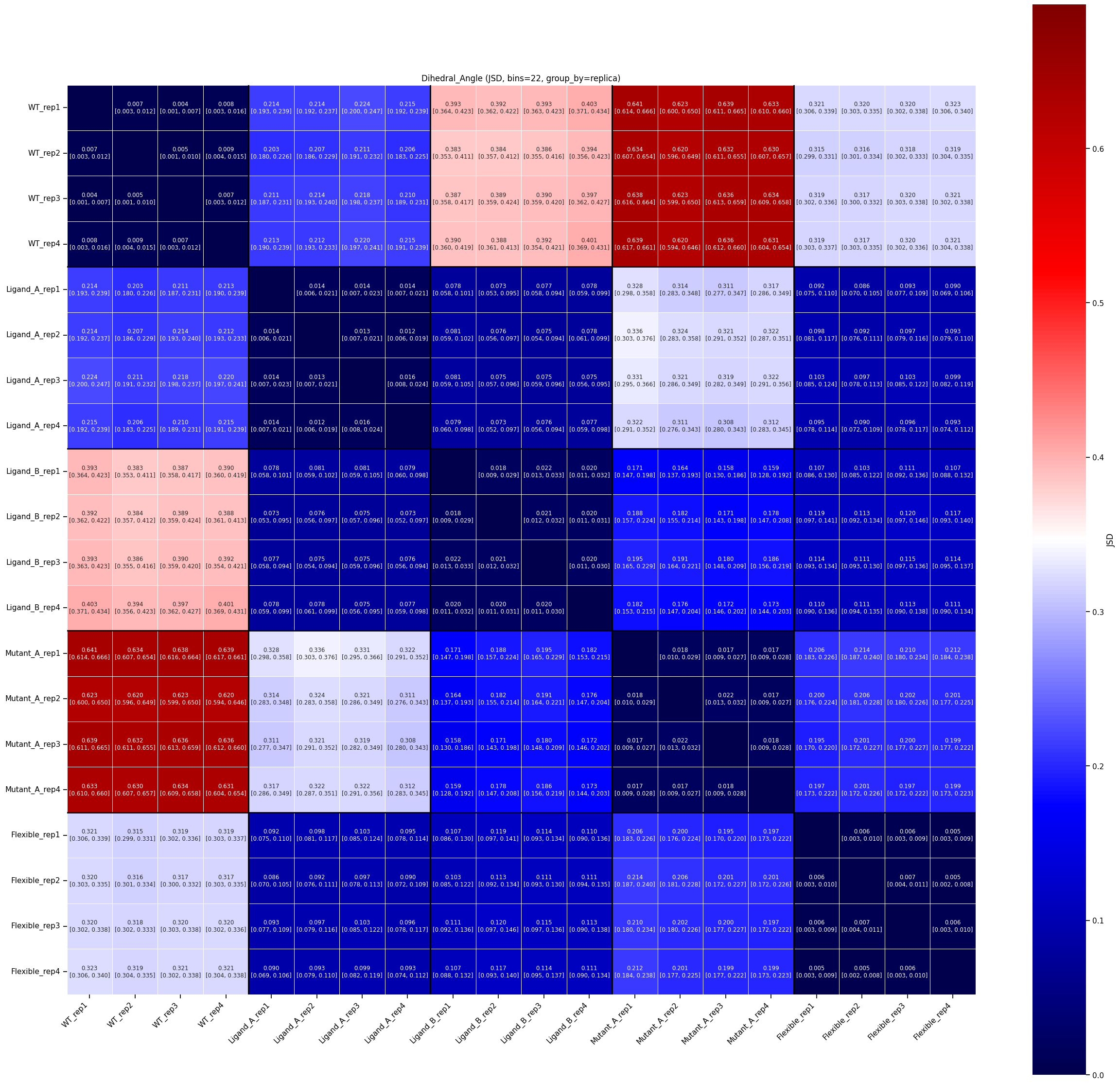
How to read the heatmap: each cell (i, j) is the inter_mean JSD between system i and system j (symmetric, diagonal = 0 by definition). The color scale runs from 0 (identical, dark blue-ish) to ln(2) ≈ 0.693 (completely non-overlapping distributions, red-ish). The two numbers printed in each cell are the mean JSD and its bootstrap confidence interval. Here every off-diagonal cell is clearly shifted from 0, and darker/warmer cells (e.g. WT vs Ligand_A) mean
a larger divergence than lighter ones (e.g. Ligand_A vs Ligand_B).
[6]:
jsd_angle = dataset.compute_jsd(
    feature_col="Dihedral_Angle", is_angle=True, plot_heatmap=True, explain=False
)
jsd_angle["system_summary"][["system_1", "system_2", "inter_mean", "verdict"]]
INFO - === Dihedral_Angle (Dihedral_Angle) | metric=jsd | group_by=replica ===
INFO - Column 'Dihedral_Angle': detected as degrees (auto)
INFO - bins: 'auto' -> 22
bootstrap JSD Dihedral_Angle: 100%|██████████| 210/210 [00:04<00:00, 43.90pair/s]
[6]:
| system_1 | system_2 | inter_mean | verdict | |
|---|---|---|---|---|
| 0 | WT | Ligand_A | 0.213058 | distinct |
| 1 | WT | Ligand_B | 0.391260 | distinct |
| 2 | WT | Mutant_A | 0.631914 | distinct |
| 3 | WT | Flexible | 0.319092 | distinct |
| 4 | Ligand_A | Ligand_B | 0.076693 | distinct |
| 5 | Ligand_A | Mutant_A | 0.319840 | distinct |
| 6 | Ligand_A | Flexible | 0.094923 | distinct |
| 7 | Ligand_B | Mutant_A | 0.176695 | distinct |
| 8 | Ligand_B | Flexible | 0.112141 | distinct |
| 9 | Mutant_A | Flexible | 0.202365 | distinct |
[7]:
jsd_pooled = dataset.compute_jsd(feature_col="RMSD", group_by="system", plot_heatmap=True)
INFO - === RMSD (RMSD) | metric=jsd | group_by=system ===
INFO - bins: 'auto' -> 44
bootstrap JSD RMSD: 100%|██████████| 15/15 [00:00<00:00, 29.83pair/s]
============================================================
                RMSD -- quick interpretation
============================================================
(bins used: 44)

+----------------------+-------------------------+----------------------+
| System pair          | JSD [95% CI]            | Magnitude (% of ln2) |
+----------------------+-------------------------+----------------------+
| WT vs Ligand_A       | 0.2788 [0.2688, 0.2906] | large (40.2%)        |
| WT vs Ligand_B       | 0.2251 [0.2145, 0.2375] | large (32.5%)        |
| WT vs Mutant_A       | 0.2091 [0.1948, 0.2229] | large (30.2%)        |
| WT vs Flexible       | 0.1616 [0.1544, 0.1705] | moderate (23.3%)     |
| Ligand_A vs Ligand_B | 0.0538 [0.0446, 0.0616] | moderate (7.8%)      |
| Ligand_A vs Mutant_A | 0.3645 [0.3448, 0.3840] | large (52.6%)        |
| Ligand_A vs Flexible | 0.1250 [0.1164, 0.1331] | moderate (18.0%)     |
| Ligand_B vs Mutant_A | 0.2240 [0.2083, 0.2392] | large (32.3%)        |
| Ligand_B vs Flexible | 0.0670 [0.0598, 0.0740] | moderate (9.7%)      |
| Mutant_A vs Flexible | 0.1366 [0.1266, 0.1489] | moderate (19.7%)     |
+----------------------+-------------------------+----------------------+

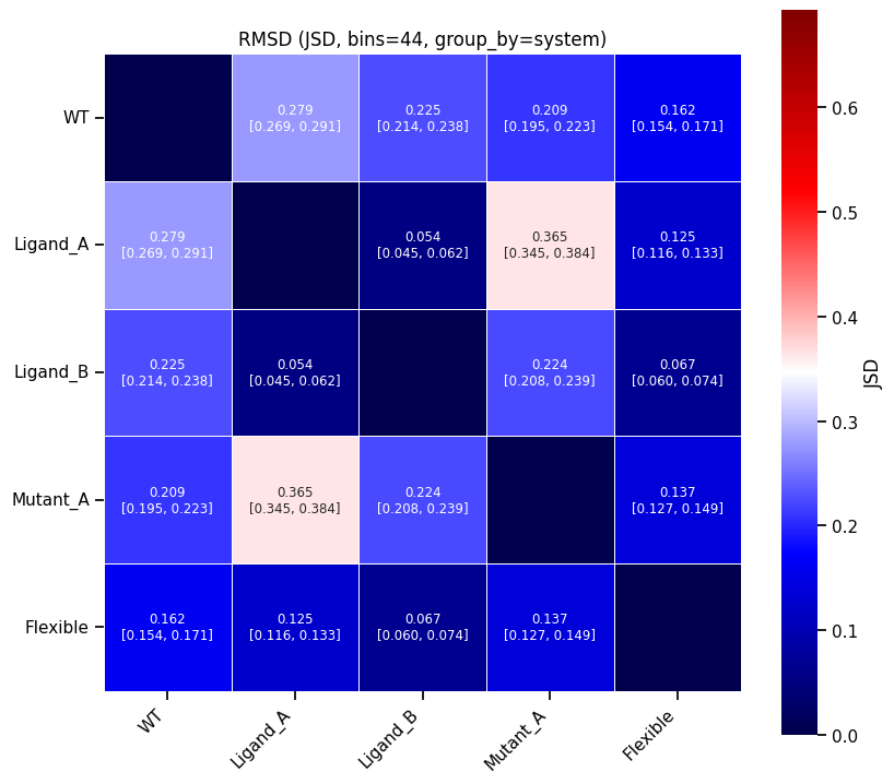
Reading guide (pooled mode -- group_by='system'): this is the raw JSD between systems with all replicas fused together. There is no
intra-system spread to compare against here, so treat the magnitude label as absolute, not as a statistically tested verdict. Re-run with
group_by='replica' (the default) for a verdict that accounts for replica-to-replica noise.

--- Table legend (see the dict for full detail) ---
+----------------+---------------------------------------------------------------------------------------------------------------------------------------------------------------------------------------------------------------------------------------------------------------------------------------------------------------------------------------------------------------------+
| Key            | What it contains                                                                                                                                                                                                                                                                                                                                                    |
+----------------+---------------------------------------------------------------------------------------------------------------------------------------------------------------------------------------------------------------------------------------------------------------------------------------------------------------------------------------------------------------------+
| system_summary | Pooled mode (group_by='system'): direct JSD between systems (all replicas fused together, one series per system). No intra-system spread, so no distinct/similar verdict -- read inter_mean/jsd_magnitude as an absolute magnitude, not a statistical test result. Switch to group_by='replica' (default) for a verdict that accounts for replica-to-replica noise. |
| bins_used      | Number of histogram bins actually used to compute the JSD (resolved from the `bins` argument -- see resolve_num_bins / resolve_bins_for_axes). Also shown in the heatmap title and in the log when verbose=True.                                                                                                                                                    |
+----------------+---------------------------------------------------------------------------------------------------------------------------------------------------------------------------------------------------------------------------------------------------------------------------------------------------------------------------------------------------------------------+
2.2 Wasserstein distance — compute_wasserstein
Same principle as compute_jsd, but using the (first-order) Wasserstein distance instead — unbounded, expressed in the feature’s native units (computed directly on the raw samples, no histogram involved). It accepts the same group_by / is_angle / iters / plot_heatmap / explain options as compute_jsd (but no bins, since no histogram is used).
[8]:
wasserstein_rmsd = dataset.compute_wasserstein(feature_col="RMSD", plot_heatmap=True)
wasserstein_rmsd["system_summary"][["system_1", "system_2", "inter_mean", "verdict"]]
INFO - === RMSD | metric=wasserstein (exact, no binning) | group_by=replica ===
bootstrap Wasserstein RMSD: 100%|██████████| 210/210 [00:08<00:00, 23.58pair/s]
============================================================
         RMSD -- quick interpretation (Wasserstein)
============================================================
(exact optimal-transport distance -- no histogram binning involved)

+----------------------+-------------------------+-----------------------+-----------------+
| System pair          | Inter distance [95% CI] | Effect ratio (95% CI) | Verdict         |
+----------------------+-------------------------+-----------------------+-----------------+
| WT vs Ligand_A       | 0.6858 [0.6374, 0.7356] | 17.06 [16.77, 17.34]  | DISTINGUISHABLE |
| WT vs Ligand_B       | 0.6358 [0.5746, 0.6982] | 13.22 [12.94, 13.49]  | DISTINGUISHABLE |
| WT vs Mutant_A       | 0.3835 [0.3304, 0.4413] | 6.56 [6.39, 6.72]     | DISTINGUISHABLE |
| WT vs Flexible       | 0.5862 [0.5362, 0.6358] | 16.21 [15.88, 16.53]  | DISTINGUISHABLE |
| Ligand_A vs Ligand_B | 0.1301 [0.0943, 0.1677] | 2.71 [2.65, 2.76]     | DISTINGUISHABLE |
| Ligand_A vs Mutant_A | 0.5302 [0.4870, 0.5754] | 9.07 [8.84, 9.29]     | DISTINGUISHABLE |
| Ligand_A vs Flexible | 0.2540 [0.2229, 0.2866] | 6.32 [6.21, 6.42]     | DISTINGUISHABLE |
| Ligand_B vs Mutant_A | 0.4573 [0.3990, 0.5171] | 7.82 [7.62, 8.02]     | DISTINGUISHABLE |
| Ligand_B vs Flexible | 0.1747 [0.1252, 0.2274] | 3.63 [3.55, 3.71]     | DISTINGUISHABLE |
| Mutant_A vs Flexible | 0.3059 [0.2646, 0.3532] | 5.23 [5.10, 5.36]     | DISTINGUISHABLE |
+----------------------+-------------------------+-----------------------+-----------------+

Reading guide: 'DISTINGUISHABLE' means the inter-system distance CI does NOT overlap either system's intra-replica (replica-to-replica) CI --
the systems differ beyond sampling noise. 'NOT distinguishable' means intra-replica noise covers the inter-system signal. 'AMBIGUOUS' overlaps
exactly one of the two intra CIs. The effect ratio is inter_mean / max(intra_1_mean, intra_2_mean) -- how many times larger the
inter-system distance is than the noisier of the two systems' own replica-to-replica spread. Values are in the feature's native units, not
a bounded [0,1]-style scale -- judge magnitude against what matters physically for this feature.

Replicas worth checking (deviate from their sisters):
+---------------+----------+---------+
| Replica       | System   | z-score |
+---------------+----------+---------+
| Ligand_B_rep2 | Ligand_B | 1.31    |
| Flexible_rep1 | Flexible | 1.24    |
+---------------+----------+---------+

--- Table legend (see the dict for full detail) ---
+------------------+-----------------------------------------------------------------------------------------------------------------------------------------------------------------------------------------------------------------------------------------------+
| Key              | What it contains                                                                                                                                                                                                                              |
+------------------+-----------------------------------------------------------------------------------------------------------------------------------------------------------------------------------------------------------------------------------------------+
| system_summary   | SYSTEM-level comparison: intra-1, intra-2, inter (mean+CI), verdict (distinct/ambiguous/similar, CI non-overlap), plus effect_ratio_*/effect_magnitude (inter/max(intra_1,intra_2)). No absolute magnitude column (Wasserstein is unbounded). |
| replica_pairs    | REPLICA-level comparison, within each system: mean+CI per replica pair.                                                                                                                                                                       |
| replica_outliers | Per REPLICA (not per pair): avg_pairwise_score, deviation_score (z-score-like vs its sisters), assessment (typical/worth_checking).                                                                                                           |
| system_overall   | Cross-feature summary: for each pair of systems, how many features say 'distinct', and an overall verdict.                                                                                                                                    |
+------------------+-----------------------------------------------------------------------------------------------------------------------------------------------------------------------------------------------------------------------------------------------+
[8]:
| system_1 | system_2 | inter_mean | verdict | |
|---|---|---|---|---|
| 0 | WT | Ligand_A | 0.685809 | distinct |
| 1 | WT | Ligand_B | 0.635807 | distinct |
| 2 | WT | Mutant_A | 0.383500 | distinct |
| 3 | WT | Flexible | 0.586193 | distinct |
| 4 | Ligand_A | Ligand_B | 0.130141 | distinct |
| 5 | Ligand_A | Mutant_A | 0.530221 | distinct |
| 6 | Ligand_A | Flexible | 0.254041 | distinct |
| 7 | Ligand_B | Mutant_A | 0.457345 | distinct |
| 8 | Ligand_B | Flexible | 0.174718 | distinct |
| 9 | Mutant_A | Flexible | 0.305851 | distinct |
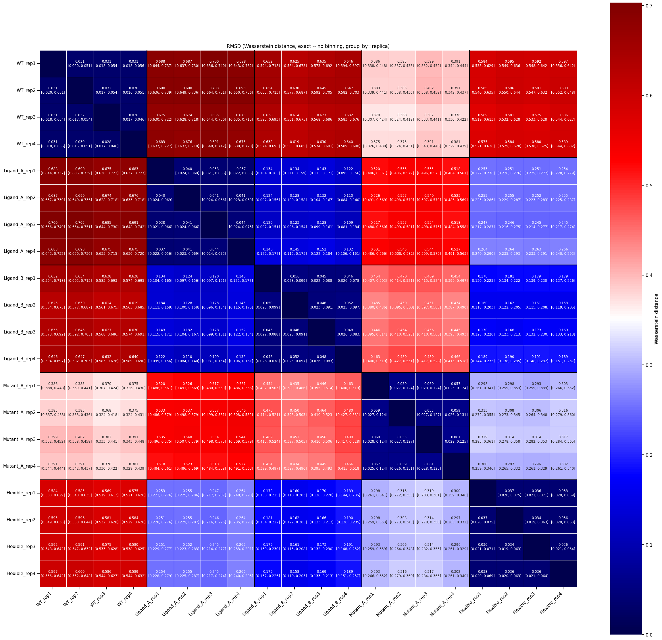
How to read this table and heatmap: same structure and same system_summary columns as compute_jsd above, but inter_mean here is a Wasserstein distance in RMSD units (not a bounded [0, ln(2)] score) – think of it as “how far do you have to shift/reshape one distribution to turn it into the other”, in the same units as the feature itself.
Because it’s unbounded, you can’t compare its absolute value across different features (a Wasserstein distance of
0.6means something different for RMSD in nm vs. an angle in degrees) – that’s exactly whatcompute_jsdis for instead.It is directly comparable within one feature though, which is useful for ranking pairs: here
WTvsLigand_A(≈0.69) is a substantially bigger shift thanLigand_AvsLigand_B(≈0.13), consistent with the JSD ranking above.The heatmap color scale is not fixed to
[0, ln(2)]like the JSD one (there’s no universal upper bound) – it auto-scales to the largest distance in the matrix, so always check the colorbar rather than comparing colors across different heatmaps.
2.3 Convergence diagnostics — compute_convergence
Checks whether a single trajectory has run long enough for a given feature to look converged (this is a per-trajectory diagnostic, not a cross-system comparison – see §2.1/2.2 for that). It reports cumulative mean/std at increasing fractions of the trajectory, a first-half-vs-second-half divergence, and a block-averaging / growing-window-JSD curve.
group_by controls how trajectories are grouped: pass ``”both”`` (system and replica together) to always get one diagnostic per actual trajectory. Using group_by="replica" alone would group by the raw replica column only – and since replica is 1, 2, 3, 4 for every system here (see the note in §1), that would silently pool WT’s replica 1 together with Mutant_A’s replica 1, Ligand_A’s replica
1, etc., as if they were one trajectory.group_by=”both”avoids that entirely by keying on(sim_name, replica)` pairs.
[9]:
convergence_all = dataset.compute_convergence(
    feature_col="RMSD", time_col="frame", group_by="both", plot=False
)
convergence_all["half_split_table"]
[9]:
| sim_name | replica | n_frames_first_half | n_frames_second_half | mean_first_half | mean_second_half | std_first_half | std_second_half | jsd_half_split | wasserstein_half_split | |
|---|---|---|---|---|---|---|---|---|---|---|
| 0 | Flexible | 1 | 720 | 720 | 2.620015 | 2.595498 | 0.719953 | 0.717061 | 0.003559 | 0.034108 |
| 1 | Flexible | 2 | 720 | 720 | 2.636631 | 2.601859 | 0.721539 | 0.719025 | 0.006441 | 0.045959 |
| 2 | Flexible | 3 | 720 | 720 | 2.637441 | 2.589661 | 0.730019 | 0.703499 | 0.003322 | 0.048308 |
| 3 | Flexible | 4 | 720 | 720 | 2.637618 | 2.607789 | 0.729956 | 0.726057 | 0.008197 | 0.044926 |
| 4 | Ligand_A | 1 | 300 | 300 | 2.694918 | 2.734150 | 0.432349 | 0.429153 | 0.014850 | 0.050136 |
| 5 | Ligand_A | 2 | 300 | 300 | 2.678206 | 2.743147 | 0.448344 | 0.421807 | 0.018137 | 0.068291 |
| 6 | Ligand_A | 3 | 300 | 300 | 2.701093 | 2.744582 | 0.448647 | 0.451846 | 0.004151 | 0.047876 |
| 7 | Ligand_A | 4 | 300 | 300 | 2.695039 | 2.729825 | 0.432664 | 0.404458 | 0.009425 | 0.051602 |
| 8 | Ligand_B | 1 | 240 | 240 | 2.767547 | 2.580003 | 0.468963 | 0.620682 | 0.108432 | 0.189468 |
| 9 | Ligand_B | 2 | 240 | 240 | 2.737917 | 2.562044 | 0.452390 | 0.646222 | 0.112279 | 0.206812 |
| 10 | Ligand_B | 3 | 240 | 240 | 2.763355 | 2.566664 | 0.470822 | 0.631334 | 0.132391 | 0.198856 |
| 11 | Ligand_B | 4 | 240 | 240 | 2.773689 | 2.567979 | 0.450316 | 0.605679 | 0.110026 | 0.206385 |
| 12 | Mutant_A | 1 | 240 | 240 | 1.918734 | 2.840604 | 0.176737 | 0.871031 | 0.248866 | 0.921899 |
| 13 | Mutant_A | 2 | 240 | 240 | 1.925143 | 2.817804 | 0.170555 | 0.912668 | 0.252534 | 0.892664 |
| 14 | Mutant_A | 3 | 240 | 240 | 1.919560 | 2.855591 | 0.167230 | 0.909029 | 0.237970 | 0.936031 |
| 15 | Mutant_A | 4 | 240 | 240 | 1.924755 | 2.861560 | 0.171685 | 0.884587 | 0.251414 | 0.937413 |
| 16 | WT | 1 | 360 | 360 | 1.921258 | 2.126453 | 0.374168 | 0.384612 | 0.046916 | 0.205310 |
| 17 | WT | 2 | 360 | 360 | 1.917302 | 2.127445 | 0.387638 | 0.383035 | 0.041051 | 0.211811 |
| 18 | WT | 3 | 360 | 360 | 1.956873 | 2.118687 | 0.394740 | 0.366950 | 0.039959 | 0.165159 |
| 19 | WT | 4 | 360 | 360 | 1.939198 | 2.128601 | 0.388197 | 0.378101 | 0.040825 | 0.190484 |
How to read ``half_split_table``: each row is one (system, replica) trajectory, split into a first half and second half. Compare mean_first_half to mean_second_half, and look at jsd_half_split/wasserstein_half_split (small = the two halves agree = converged; large = the trajectory is still drifting).
Looking at the table above:
``Flexible`` and ``Ligand_A`` are well converged: the mean barely moves between halves, and
jsd_half_splitstays tiny (≈0.003–0.02, i.e. well under 5% of theln(2)≈0.693maximum).``WT`` is borderline-good: a small but consistent shift (
jsd_half_split ≈0.04–0.05across all 4 replicas).``Mutant_A`` is a red flag: the mean RMSD jumps from
≈1.92in the first half to≈2.85in the second half, for every replica, withjsd_half_split ≈0.24–0.25(over a third of the maximum possible value) and a largewasserstein_half_split(≈0.9, vs.≈0.03forFlexible). That’s a consistent, systematic drift, not noise – this system’s trajectories don’t look converged for RMSD, and you’d want to extend the simulation (or discard the first part as equilibration) before trusting downstream comparisons involvingMutant_A.
Let’s visualize that contrast directly with plot=True, filtered to the problematic system:
[10]:
convergence_mutant = dataset.compute_convergence(
    feature_col="RMSD", time_col="frame", sim_name="Mutant_A", group_by="both", plot=True
)
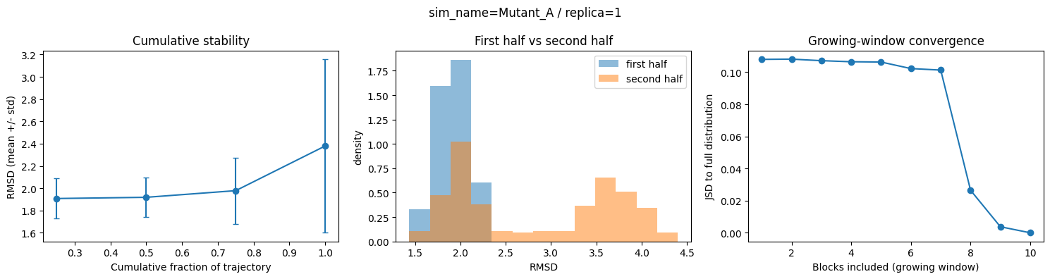
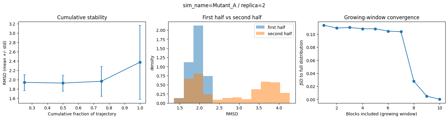
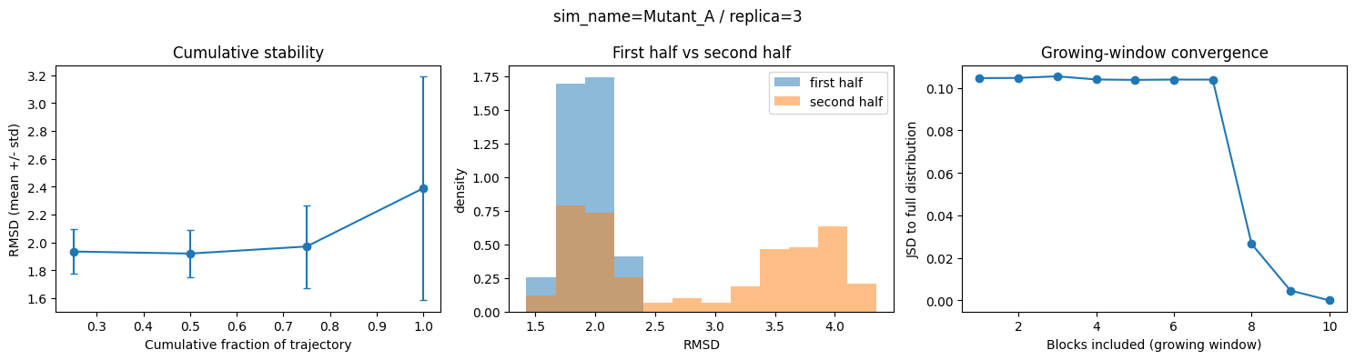
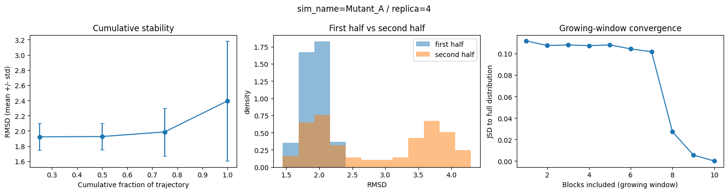
How to read the 3-panel figures above (one figure per Mutant_A replica):
Left (“Cumulative stability”): mean +/- std of RMSD computed on the first 25%, 50%, 75%, 100% of the trajectory. For
Mutant_Athe mean visibly climbs as more of the trajectory is included instead of flattening out – the signature of a trajectory that hasn’t plateaued yet.Middle (“First half vs second half”): histograms of the first half (blue) and second half (orange) overlaid. For a converged trajectory these two histograms should look like near-identical copies of each other. Here they’re clearly shifted apart – visual confirmation of the large
jsd_half_splitfrom the table above.Right (“Growing-window convergence”): JSD between “everything seen so far” (after including 1, 2, …, 10 blocks) and the full trajectory’s distribution. It should drop toward 0 quickly and stay there. Compare this curve for
Mutant_Ato the one you’d get forFlexiblebelow – it takes much longer to flatten out, and/or doesn’t flatten as low.
[11]:
convergence_flexible = dataset.compute_convergence(
    feature_col="RMSD", time_col="frame", sim_name="Flexible", replica=1, group_by="both", plot=True
)
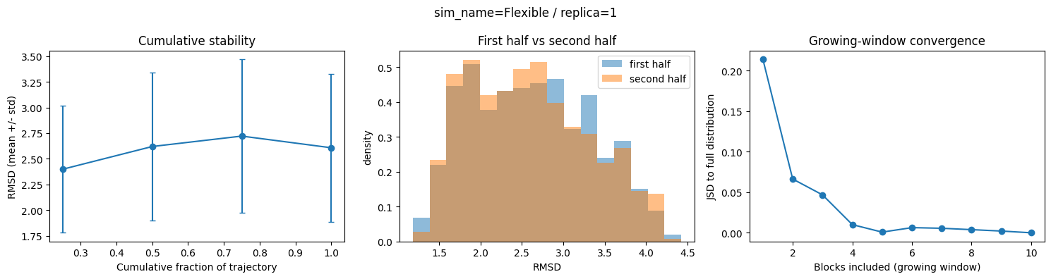
Compare the two sets of figures: Flexible’s cumulative mean is flat from the start, its first/second-half histograms overlap almost perfectly, and its growing-window JSD collapses to ~0 within the first couple of blocks – a textbook example of a converged trajectory, right next to Mutant_A’s non-converged one.
3. Clustering
RepLikCompare wraps several clustering algorithms behind a consistent interface: pass a set of numeric feature_cols, get back the original DataFrame with an added cluster column plus any diagnostic figures.
3.1 K-means — compute_cluster_kmean
Main options:
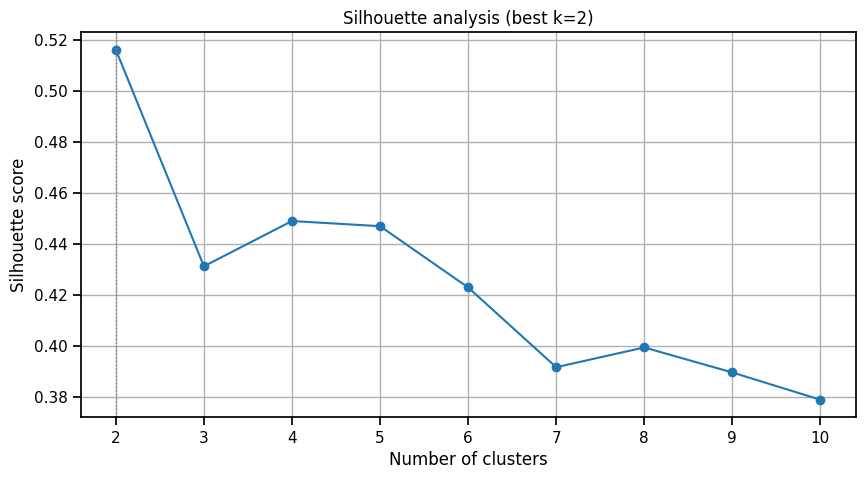
max_cluster(default20): upper bound of the silhouette search (used whenncluster=None).ncluster: if given, skips the search and uses thiskdirectly.random_state,n_init,max_iter: forwarded toKMeans.silhouette_plot(defaultTrue): compute and return the silhouette-vs-k curve (only meaningful whenncluster=None).context,figsize: styling of the silhouette figure.
Returns: (new_df, figures) — figures contains "silhouette" if a search was performed, otherwise {}.
[12]:
feature_cols = ["Radius_Gyration", "SASA", "RMSD", "HBonds", "Potential_Energy"]
new_df, figures = dataset.compute_cluster_kmean(feature_cols=feature_cols, max_cluster=10)
figures["silhouette"]
INFO - KMeans parameters: n_init=10, max_iter=300, random_state=0
INFO - No ncluster provided, testing from 2 to 10 clusters.
INFO - Testing k = 2
INFO - Testing k = 3
INFO - Testing k = 4
INFO - Testing k = 5
INFO - Testing k = 6
INFO - Testing k = 7
INFO - Testing k = 8
INFO - Testing k = 9
INFO - Testing k = 10
INFO - Optimal number of clusters: 2 (silhouette = 0.516)
INFO - Kmeans clustering completed. Number of clusters: 2
INFO - Cluster:  1    5347 |  35.93%
INFO - Cluster:  2    9533 |  64.07%
[12]:
[13]:
new_df, figures = dataset.compute_cluster_kmean(feature_cols=feature_cols, ncluster=6, silhouette_plot=False)
dataset.df = new_df.rename(columns={"cluster": "kmeans_cluster"})
dataset.df[["sim_name", "replica", "kmeans_cluster"]].head()
INFO - KMeans parameters: n_init=10, max_iter=300, random_state=0
INFO - Using ncluster = 6
INFO - Kmeans clustering completed. Number of clusters: 6
INFO - Cluster:  1    1423 |   9.56%
INFO - Cluster:  2    2516 |  16.91%
INFO - Cluster:  3    2030 |  13.64%
INFO - Cluster:  4    2039 |  13.70%
INFO - Cluster:  5    3723 |  25.02%
INFO - Cluster:  6    3149 |  21.16%
[13]:
| sim_name | replica | kmeans_cluster | |
|---|---|---|---|
| 0 | WT | 1 | 2 |
| 1 | WT | 1 | 2 |
| 2 | WT | 1 | 5 |
| 3 | WT | 1 | 2 |
| 4 | WT | 1 | 2 |
3.2 Gaussian Mixture Model — compute_cluster_GMM
Same conventions as K-means, plus:
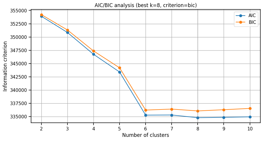
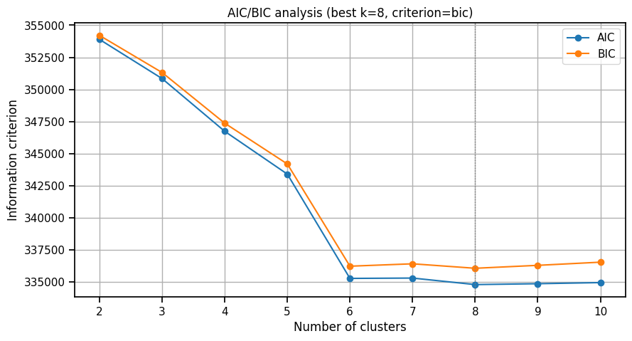
min_cluster(default1): lower bound of the search.covariance_type:"full"/"tied"/"diag"/"spherical".criterion:"aic"or"bic"(the minimum is best, unlike the silhouette score).ic_plot(instead ofsilhouette_plot): AIC/BIC-vs-k figure.tol,reg_covar,init_params,n_init,max_iter: EM parameters.
Returns: figures contains "aic_bic" if a search was performed.
[14]:
new_df, figures = dataset.compute_cluster_GMM(
    feature_cols=feature_cols, min_cluster=2, max_cluster=10, criterion="bic"
)
figures["aic_bic"]
INFO - GMM parameters: covariance_type=full, n_init=1, max_iter=100, random_state=0
INFO - No ncluster provided, testing from 2 to 10 clusters (criterion=bic).
INFO - Testing k = 2
INFO - Testing k = 3
INFO - Testing k = 4
INFO - Testing k = 5
INFO - Testing k = 6
INFO - Testing k = 7
INFO - Testing k = 8
INFO - Testing k = 9
INFO - Testing k = 10
INFO - Optimal number of clusters: 8 (bic = 336076.004)
INFO - GMM converged: True (n_iter=10)
INFO - GMM clustering completed. Number of clusters: 8
INFO - Cluster:  1     342 |   2.30%
INFO - Cluster:  2    2849 |  19.15%
INFO - Cluster:  3     433 |   2.91%
INFO - Cluster:  4    1404 |   9.44%
INFO - Cluster:  5    2678 |  18.00%
INFO - Cluster:  6    1020 |   6.85%
INFO - Cluster:  7    4101 |  27.56%
INFO - Cluster:  8    2053 |  13.80%
INFO - GMM means shape: (8, 5)
[14]:
3.3 Hierarchical clustering — hierarchical_clustering
Agglomerative hierarchical clustering (scipy.cluster.hierarchy), with a few extra options:
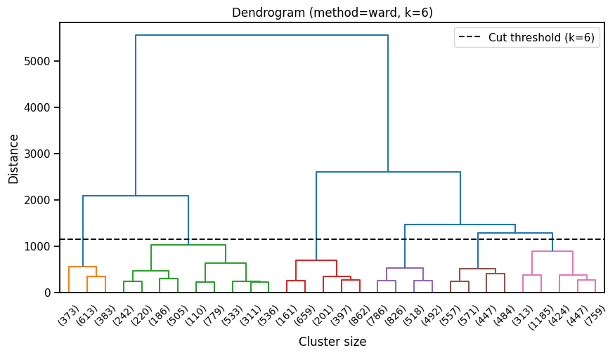
method/metric: forwarded tolinkage(e.g."ward"/"euclidean").max_data: subsample if there are more rows than this (linkage is expensive in memory/time on large datasets).dendrogram_plot(defaultTrue): draw the dendrogram.truncate_mode,p: dendrogram display options (scipy.dendrogram).
Returns: figures may contain "silhouette" and/or "dendrogram".
[15]:
new_df, figures = dataset.hierarchical_clustering(
    feature_cols=feature_cols, ncluster=6, silhouette_plot=False, dendrogram_plot=True
)
INFO - HAC parameters: method=ward, metric=euclidean (forced by ward), n_samples=14880
INFO - Computing linkage matrix...
INFO - Using ncluster = 6
INFO - HAC clustering completed. Number of clusters: 6
INFO - Cluster:  1    1369 |   9.20%
INFO - Cluster:  2    3422 |  23.00%
INFO - Cluster:  3    2280 |  15.32%
INFO - Cluster:  4    2622 |  17.62%
INFO - Cluster:  5    2059 |  13.84%
INFO - Cluster:  6    3128 |  21.02%
3.4 DBSCAN — compute_cluster_dbscan
Density-based clustering — detects noise natively.
eps: neighborhood radius.min_samples: minimum number of points to form a dense cluster.
There is no search over k (DBSCAN doesn’t need one), so ``figures`` is always ``{}``. Noise is labeled -1 (scikit-learn convention); real clusters are renumbered 1..k by decreasing population.
[16]:
new_df, figures = dataset.compute_cluster_dbscan(feature_cols=feature_cols, eps=3.0, min_samples=30)
dataset.df = new_df.rename(columns={"cluster": "dbscan_cluster"})
dataset.df[["sim_name", "replica", "dbscan_cluster"]].head()
INFO - Number of clusters: 7, unclustered (noise) points: 36.8%
INFO - Noise (-1)      5478 |  36.81%
INFO - Cluster 1       5600 |  37.63%
INFO - Cluster 2       1906 |  12.81%
INFO - Cluster 3       1465 |   9.85%
INFO - Cluster 4        317 |   2.13%
INFO - Cluster 5         53 |   0.36%
INFO - Cluster 6         36 |   0.24%
INFO - Cluster 7         25 |   0.17%
INFO - DBSCAN clustering completed. Number of clusters: 7
[16]:
| sim_name | replica | dbscan_cluster | |
|---|---|---|---|
| 0 | WT | 1 | 3 |
| 1 | WT | 1 | 3 |
| 2 | WT | 1 | -1 |
| 3 | WT | 1 | 3 |
| 4 | WT | 1 | 3 |
3.5 HDBSCAN — compute_cluster_hdbscan
Hierarchical density-based clustering — no need to fix eps.
min_cluster_size: minimum size of a cluster.min_samples: controls sensitivity to noise (higher = more noise).
Same -1 noise convention, same figures = {}.
[17]:
new_df, figures = dataset.compute_cluster_hdbscan(
    feature_cols=feature_cols, min_cluster_size=80, min_samples=30
)
dataset.df = new_df.rename(columns={"cluster": "hdbscan_cluster"})
INFO - Number of clusters: 2, unclustered (noise) points: 5.3%
INFO - Noise (-1)       791 |   5.32%
INFO - Cluster 1      12936 |  86.94%
INFO - Cluster 2       1153 |   7.75%
INFO - HDBSCAN clustering completed. Number of clusters: 2
3.6 Cluster representatives — assign_cluster_representative
Picks one representative frame per cluster (closest to the centroid/medoid), from an already-computed cluster column.
Main options:
cluster_col,feature_cols: the cluster column plus the numeric columns used for distance.group_by:"sim_name"(one representative per system),"replica"(per replica — usesunique_replica_colinternally, so it stays correct even whenreplicalabels are reused across systems),"both"(per system and replica), orNone(global, if clustering was done on the wholeDatasetat once).method:"centroid"(point closest to the cluster mean) or"medoid"(point minimizing the total distance to other points in the cluster — more robust to non-convex clusters, more expensive).noise_label(default-1): value ofcluster_colto exclude (set toNoneif there is no noise label, e.g. K-means/GMM).include_distance: add adistance_to_referencecolumn.
Returns: a DataFrame with one row per (group, cluster), with columns frame_index (the original index in dataset.df, to look up the full frame via dataset.df.loc[frame_index]), cluster_size, and distance_to_reference.
[18]:
hdbscan_reps_by_replica = dataset.assign_cluster_representative(
    cluster_col="hdbscan_cluster", feature_cols=feature_cols,
    group_by="replica", method="medoid", noise_label=None,
)
print(f"{len(hdbscan_reps_by_replica)} representatives (one per system/replica)")
hdbscan_reps_by_replica.head()
48 representatives (one per system/replica)
[18]:
| System | hdbscan_cluster | frame_index | cluster_size | distance_to_reference | |
|---|---|---|---|---|---|
| 0 | Flexible_rep1 | -1 | 9791 | 88 | 50.965057 |
| 1 | Flexible_rep1 | 1 | 9956 | 1152 | 33.783719 |
| 2 | Flexible_rep1 | 2 | 9839 | 200 | 12.473433 |
| 3 | Flexible_rep2 | -1 | 11169 | 100 | 53.871182 |
| 4 | Flexible_rep2 | 1 | 11501 | 1140 | 33.671247 |
[19]:
hdbscan_reps_by_system = dataset.assign_cluster_representative(
    cluster_col="hdbscan_cluster", feature_cols=feature_cols,
    group_by="sim_name", method="medoid", noise_label=None,
)
print(f"{len(hdbscan_reps_by_system)} representatives (one per system)")
hdbscan_reps_by_system.head()
12 representatives (one per system)
[19]:
| sim_name | hdbscan_cluster | frame_index | cluster_size | distance_to_reference | |
|---|---|---|---|---|---|
| 0 | Flexible | -1 | 13399 | 413 | 52.322078 |
| 1 | Flexible | 1 | 14338 | 4559 | 33.736819 |
| 2 | Flexible | 2 | 13970 | 788 | 12.157152 |
| 3 | Ligand_A | -1 | 4181 | 67 | 31.714872 |
| 4 | Ligand_A | 1 | 3355 | 2333 | 24.703639 |
4. Dimensionality reduction
4.1 PCA — compute_pca
[20]:
pca_df, pca_fig, pca_model = dataset.compute_pca(feature_cols=feature_cols, n_components=3, s=50)
print("Explained variance ratio:", pca_model.explained_variance_ratio_)
pca_df.head()
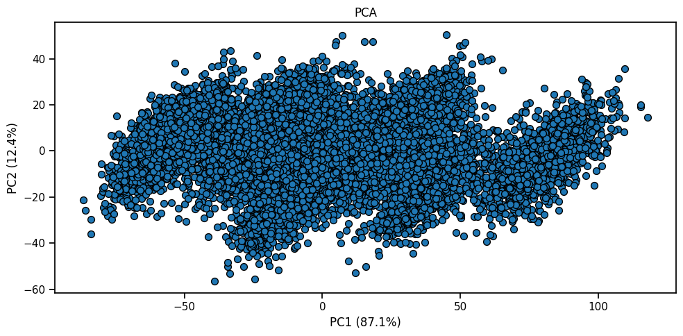
INFO - Running PCA with n_components=3
INFO - PC1 explained variance ratio: 87.13%
INFO - PC2 explained variance ratio: 12.41%
INFO - PC3 explained variance ratio: 0.42%
INFO - PCA completed. Total explained variance: 99.96%
INFO - Plotting PCA results...
Explained variance ratio: [0.8713174 0.12410242 0.00421868]
[20]:
| sim_name | replica | frame | cluster_state | Radius_Gyration | SASA | RMSD | RMSF | HBonds | Potential_Energy | Dihedral_Angle | System | kmeans_cluster | dbscan_cluster | hdbscan_cluster | PC1 | PC2 | PC3 | |
|---|---|---|---|---|---|---|---|---|---|---|---|---|---|---|---|---|---|---|
| 0 | WT | 1 | 0 | 0 | 18.120029 | 162.326932 | 1.584457 | 0.662354 | 205.009943 | -1373.041538 | -96.400189 | WT_rep1 | 2 | 3 | 1 | -46.029020 | 15.848941 | 2.219929 |
| 1 | WT | 1 | 1 | 0 | 18.349881 | 156.711960 | 1.872718 | 0.773739 | 202.541489 | -1383.147669 | -51.348810 | WT_rep1 | 2 | 3 | 1 | -55.664571 | 11.171362 | -2.710353 |
| 2 | WT | 1 | 2 | 0 | 19.272076 | 176.338459 | 2.095835 | 0.833684 | 206.182798 | -1369.002222 | -74.037508 | WT_rep1 | 5 | -1 | 1 | -32.228127 | 11.374830 | 4.367427 |
| 3 | WT | 1 | 3 | 0 | 18.911540 | 159.142525 | 1.671309 | 0.713268 | 207.590998 | -1404.957461 | -86.691822 | WT_rep1 | 2 | 3 | 1 | -65.614091 | -8.980824 | -3.336021 |
| 4 | WT | 1 | 4 | 0 | 17.879963 | 152.160358 | 1.597107 | 0.730884 | 207.234531 | -1385.006682 | -73.193045 | WT_rep1 | 2 | 3 | 1 | -61.122452 | 11.090542 | 1.361457 |
4.2 UMAP / t-SNE / kernel PCA
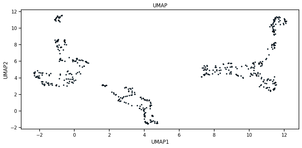
Unlike PCA, these methods scale poorly with the number of points, so we work on a random subsample here.
[21]:
X_sub = dataset.df[feature_cols].sample(n=500, random_state=0)
print("X_sub:", X_sub.shape)

sub_dataset = rlc.Dataset.from_dataframe(X_sub)
WARNING - Dataset: couldn't auto-detect a simulation-name column (tried ('sim_name', 'sim', 'system', 'system_name', 'SIM_NAME', 'SIM', 'SYSTEM', 'SYSTEM_NAME', 'simulation', 'simulation_name', 'SIMULATION', 'SIMULATION_NAME', 'simulation_name', 'simulation_id', 'SIMULATION_ID', 'SIMULATION_NAME', 'simulation_identifier', 'SIMULATION_IDENTIFIER', 'simulation_identification', 'SIMULATION_IDENTIFICATION', 'simulation_ident', 'SIMULATION_IDENT', 'simulation_ind', 'SIMULATION_IND', 'simulation_index', 'SIMULATION_INDEX', 'simulation_idx', 'SIMULATION_IDX', 'simulation_number', 'SIMULATION_NUMBER', 'simulation_num', 'SIMULATION_NUM', 'simulation_indx', 'SIMULATION_INDX', 'simulation_ind', 'SIMULATION_IND', 'simulation_id_num', 'SIMULATION_ID_NUM', 'simulation_identification', 'SIMULATION_IDENTIFICATION', 'simulation_identifier', 'SIMULATION_IDENTIFIER', 'simulation_ident', 'SIMULATION_IDENT', 'simulation_ind', 'SIMULATION_IND', 'simulation_index', 'SIMULATION_INDEX', 'simulation_idx', 'SIMULATION_IDX', 'simulation_number', 'SIMULATION_NUMBER', 'simulation_num', 'SIMULATION_NUM', 'simulation_indx', 'SIMULATION_INDX', 'simulation_ind', 'SIMULATION_IND', 'simulation_id_num', 'SIMULATION_ID_NUM', 'simulation_identification', 'SIMULATION_IDENTIFICATION', 'simulation_identifier', 'SIMULATION_IDENTIFIER', 'simulation_ident', 'SIMULATION_IDENT', 'simulation_ind', 'SIMULATION_IND', 'simulation_index', 'SIMULATION_INDEX', 'simulation_idx', 'SIMULATION_IDX', 'simulation_number', 'SIMULATION_NUMBER', 'simulation_num', 'SIMULATION_NUM', 'simulation_indx', 'SIMULATION_INDX')). Please specify it explicitly, e.g. Dataset.from_csv(path, sim_name_col='sim_name', replica_col='replica'). Methods that need it will raise a clear error until then.
WARNING - Dataset: couldn't auto-detect a replica column (tried ('replica', 'rep', 'replicate', 'REPLICA', 'REP', 'REPLICATE', 'replica_id', 'rep_id', 'REPLICA_ID', 'REP_ID', 'replicate_id', 'REPLICATE_ID', 'replica_name', 'rep_name', 'REPLICA_NAME', 'REP_NAME', 'replicate_name', 'REPLICATE_NAME', 'replica_num', 'rep_num', 'REPLICA_NUM', 'REP_NUM', 'replicate_num', 'REPLICATE_NUM', 'replica_index', 'rep_index', 'REPLICA_INDEX', 'REP_INDEX', 'replicate_index', 'REPLICATE_INDEX', 'replica_idx', 'rep_idx', 'REPLICA_IDX', 'REP_IDX', 'replicate_idx', 'REPLICATE_IDX', 'replica_number', 'rep_number', 'REPLICA_NUMBER', 'REP_NUMBER', 'replicate_number', 'REPLICATE_NUMBER', 'replica_indx', 'rep_indx', 'REPLICA_INDX', 'REP_INDX', 'replicate_indx', 'REPLICATE_INDX', 'replica_ind', 'rep_ind', 'REPLICA_IND', 'REP_IND', 'replicate_ind', 'REPLICATE_IND', 'replica_id_num', 'rep_id_num', 'REPLICA_ID_NUM', 'REP_ID_NUM', 'replicate_id_num', 'REPLICATE_ID_NUM', 'replica_identifier', 'rep_identifier', 'REPLICA_IDENTIFIER', 'REP_IDENTIFIER', 'replicate_identifier', 'REPLICATE_IDENTIFIER', 'replica_ident', 'rep_ident', 'REPLICA_IDENT', 'REP_IDENT', 'replicate_ident', 'REPLICATE_IDENT', 'replica_identification', 'rep_identification', 'REPLICA_IDENTIFICATION', 'REP_IDENTIFICATION', 'replicate_identification', 'REPLICATE_IDENTIFICATION')). Please specify it explicitly, e.g. Dataset.from_csv(path, sim_name_col='sim_name', replica_col='replica'). Methods that need it will raise a clear error until then.
X_sub: (500, 5)
[22]:
# UMAP
umap_df, umap_fig, umap_model = sub_dataset.compute_umap(
    feature_cols=feature_cols, n_neighbors=15, min_dist=0.1, random_state=0,
)
display(umap_df.head())

# t-SNE
tsne_df, tsne_fig, tsne_model = sub_dataset.compute_tsne(
    feature_cols=feature_cols, perplexity=30, random_state=0,
)
display(tsne_df.head())

# Kernel PCA
kpca_df, kpca_fig, kpca_model = sub_dataset.compute_kpca(
    feature_cols=feature_cols, n_components=3, kernel="rbf",
)
display(kpca_df.head())
INFO - Running UMAP with n_neighbors=15, min_dist=0.100, metric=euclidean
UMAP(n_jobs=1, random_state=0, verbose=True)
Thu Aug 13 09:46:48 2026 Construct fuzzy simplicial set
/usr/local/lib/python3.12/dist-packages/umap/umap_.py:1952: UserWarning: n_jobs value 1 overridden to 1 by setting random_state. Use no seed for parallelism.
  warn(
Thu Aug 13 09:46:48 2026 Finding Nearest Neighbors
Thu Aug 13 09:46:53 2026 Finished Nearest Neighbor Search
Thu Aug 13 09:46:57 2026 Construct embedding
Epochs completed: 16%| █▌ 81/500 [00:00]
        completed  0  /  500 epochs
        completed  50  /  500 epochs
        completed  100  /  500 epochs
        completed  150  /  500 epochs
Epochs completed: 63%| ██████▎ 314/500 [00:01]
        completed  200  /  500 epochs
        completed  250  /  500 epochs
        completed  300  /  500 epochs
        completed  350  /  500 epochs
Epochs completed: 100%| ██████████ 500/500 [00:01]
INFO - UMAP completed.
INFO - Plotting UMAP results...
        completed  400  /  500 epochs
        completed  450  /  500 epochs
Thu Aug 13 09:46:59 2026 Finished embedding
| Radius_Gyration | SASA | RMSD | HBonds | Potential_Energy | UMAP1 | UMAP2 | |
|---|---|---|---|---|---|---|---|
| 7291 | 19.591989 | 210.693401 | 1.949451 | 199.127566 | -1381.960330 | 3.927661 | 0.379179 |
| 1283 | 18.777694 | 167.586120 | 1.894782 | 207.357071 | -1396.122055 | 12.073458 | 10.818481 |
| 6353 | 21.604540 | 214.963411 | 2.717643 | 196.196942 | -1352.933240 | 1.794968 | 3.090078 |
| 13135 | 20.627813 | 189.198020 | 2.677428 | 193.844822 | -1351.898543 | 11.438584 | 3.309087 |
| 220 | 20.631296 | 181.965174 | 2.452151 | 199.128410 | -1367.553521 | 10.339742 | 5.902302 |
INFO - Running t-SNE with perplexity=30, metric=euclidean
[t-SNE] Computing 91 nearest neighbors...
[t-SNE] Indexed 500 samples in 0.001s...
[t-SNE] Computed neighbors for 500 samples in 0.007s...
[t-SNE] Computed conditional probabilities for sample 500 / 500
[t-SNE] Mean sigma: 6.946303
[t-SNE] KL divergence after 250 iterations with early exaggeration: 39.868668
INFO - t-SNE completed.
INFO - Plotting t-SNE results...
[t-SNE] KL divergence after 2250 iterations: 0.322040
| Radius_Gyration | SASA | RMSD | HBonds | Potential_Energy | TSNE1 | TSNE2 | |
|---|---|---|---|---|---|---|---|
| 7291 | 19.591989 | 210.693401 | 1.949451 | 199.127566 | -1381.960330 | 1.693711 | 10.232561 |
| 1283 | 18.777694 | 167.586120 | 1.894782 | 207.357071 | -1396.122055 | 37.695873 | -11.956956 |
| 6353 | 21.604540 | 214.963411 | 2.717643 | 196.196942 | -1352.933240 | -11.238180 | 2.063724 |
| 13135 | 20.627813 | 189.198020 | 2.677428 | 193.844822 | -1351.898543 | 8.077787 | -16.545376 |
| 220 | 20.631296 | 181.965174 | 2.452151 | 199.128410 | -1367.553521 | 18.673439 | -11.139412 |
INFO - Running KPCA with kernel=rbf
INFO - KPCA completed.
INFO - Plotting KPCA results...
| Radius_Gyration | SASA | RMSD | HBonds | Potential_Energy | KPC1 | KPC2 | KPC3 | |
|---|---|---|---|---|---|---|---|---|
| 7291 | 19.591989 | 210.693401 | 1.949451 | 199.127566 | -1381.960330 | -0.010413 | -0.003944 | -0.003467 |
| 1283 | 18.777694 | 167.586120 | 1.894782 | 207.357071 | -1396.122055 | -0.019842 | -0.012520 | -0.017632 |
| 6353 | 21.604540 | 214.963411 | 2.717643 | 196.196942 | -1352.933240 | -0.009776 | -0.003521 | -0.003059 |
| 13135 | 20.627813 | 189.198020 | 2.677428 | 193.844822 | -1351.898543 | -0.011120 | -0.004128 | -0.003597 |
| 220 | 20.631296 | 181.965174 | 2.452151 | 199.128410 | -1367.553521 | 0.058403 | -0.000608 | -0.006776 |
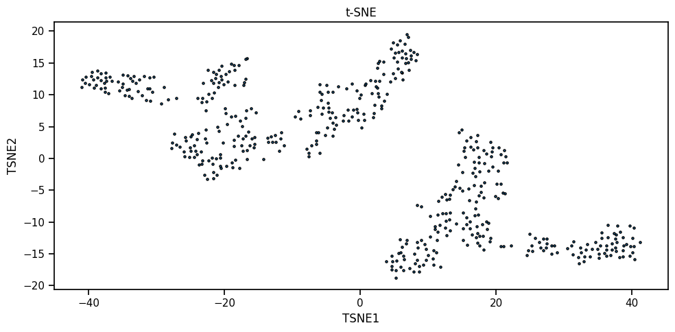
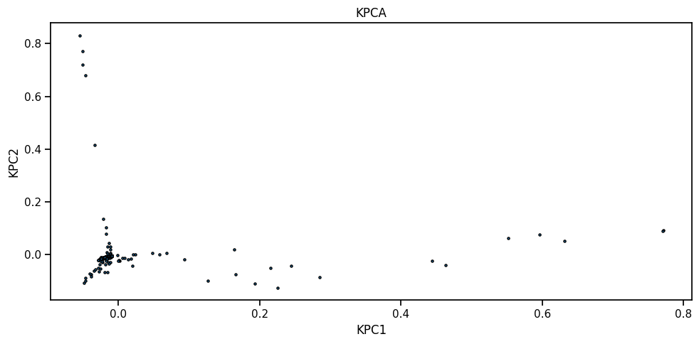
5. Plotting
Every plot below is available both as a standalone function and as a Dataset method of the same name (used here) — see the Plotting page for the full reference.
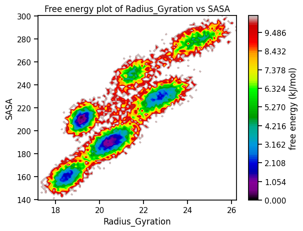
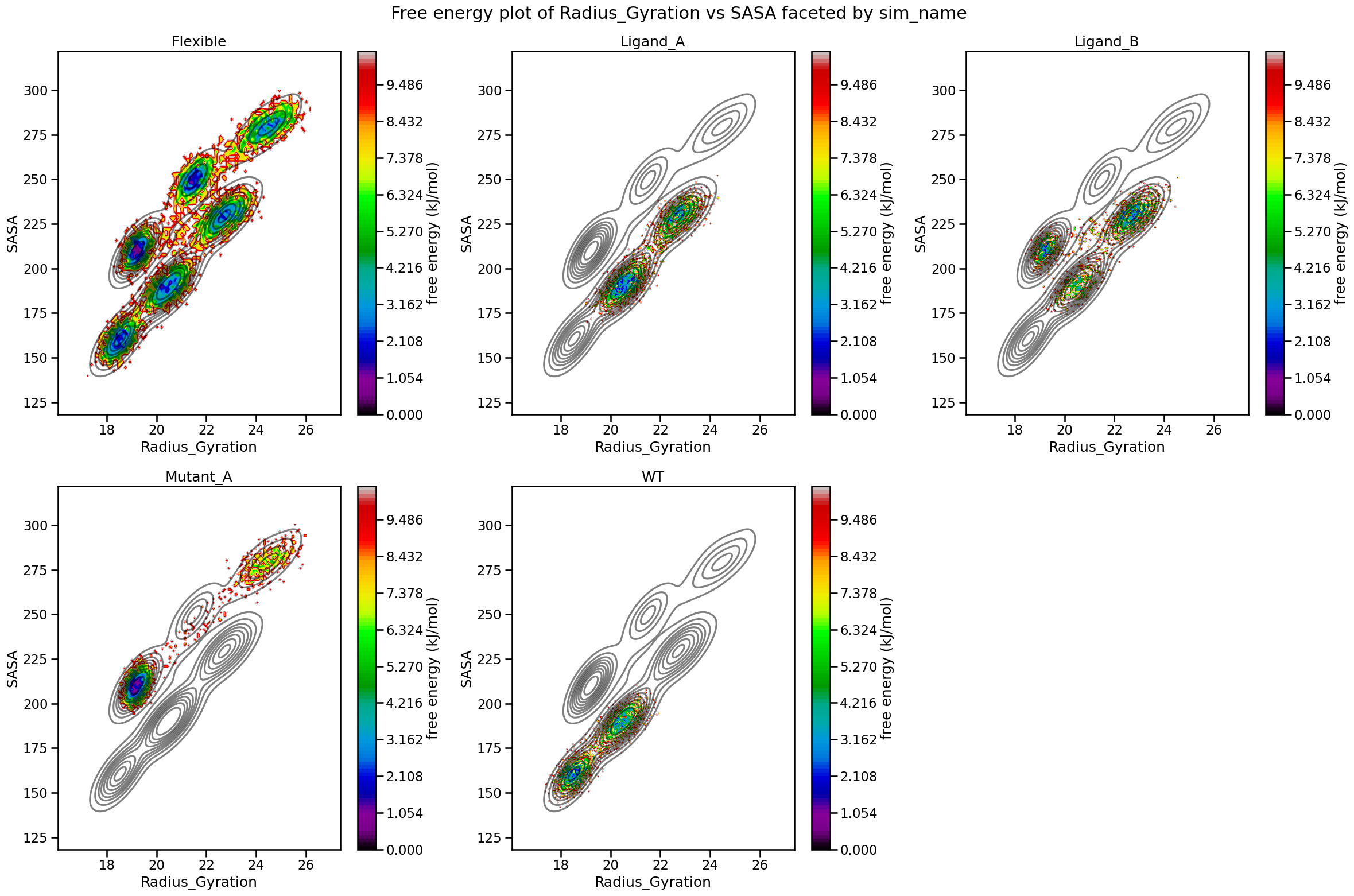
5.1 Free-energy landscapes — plot_free_energy / plot_free_energy_facet
[23]:
fig, ax, misc = dataset.plot_free_energy(x="Radius_Gyration", y="SASA", context="notebook")
[24]:
fig, axes, miscs = dataset.plot_free_energy_facet(
    x="Radius_Gyration", y="SASA", facet_col="sim_name", ncols=3, global_density=True,
)
5.2 Replica-averaged line plots — plot_lineplot_avg / plot_lineplot_facet
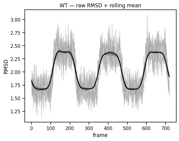
[25]:
ax = dataset.plot_lineplot_avg(x="frame", y="RMSD", sim_name="WT", avg_win=15)
plt.title("WT — raw RMSD + rolling mean")
plt.show()
[26]:
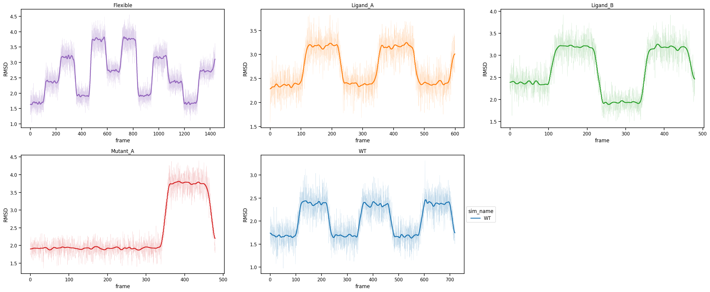
fig, axes = dataset.plot_lineplot_facet(
    x="frame", y="RMSD", facet_col="sim_name", ncols=3, avg_win=15,
)
5.3 Distributions — plot_distri_norm
[27]:
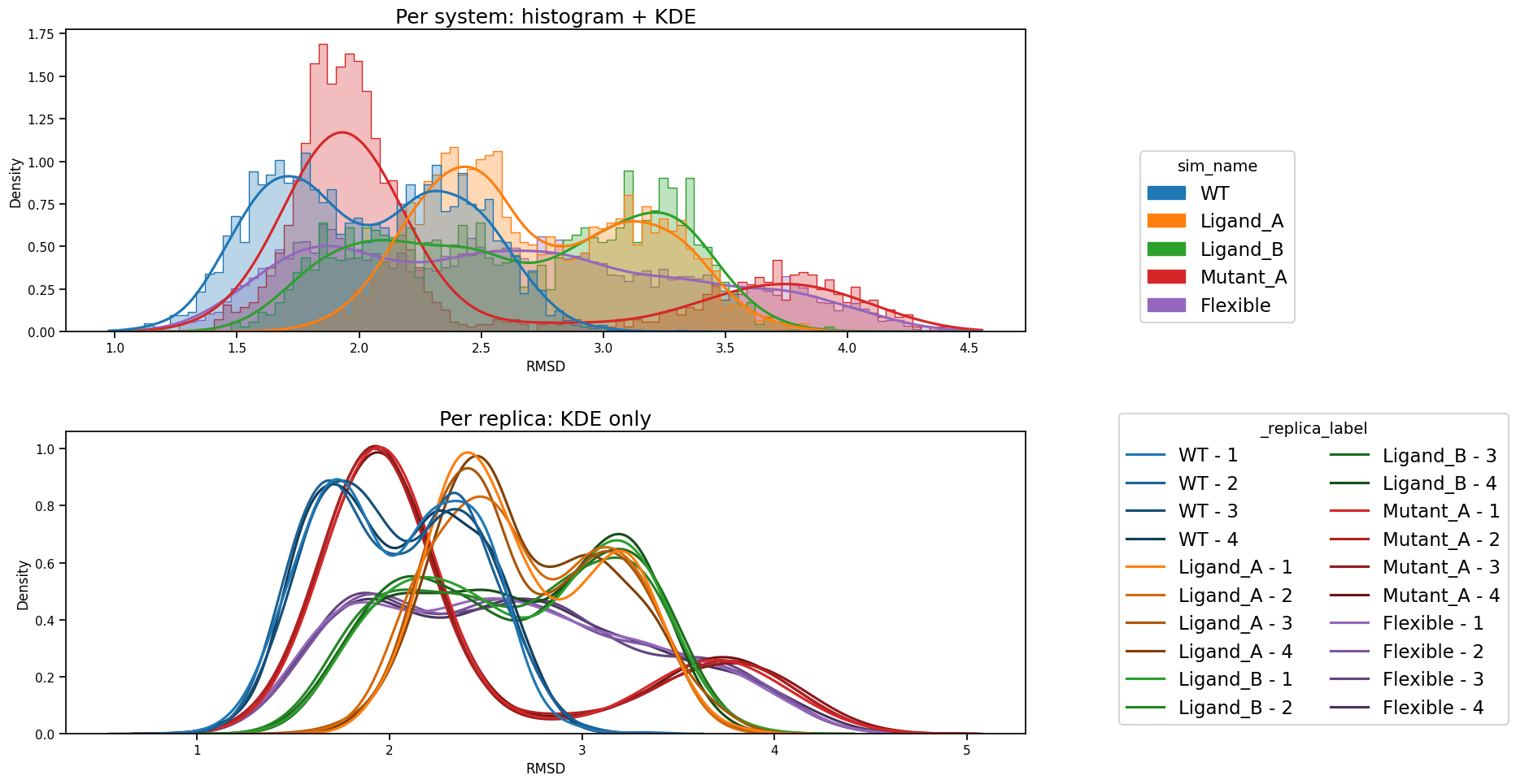
fig, axes = plt.subplots(2, 1, figsize=(20, 10))

dataset.plot_distri_norm(x="RMSD", mode="per_sim", fill=True, alpha=0.3, bw_adjust=1.0, ax=axes[0])
dataset.plot_distri_norm(x="RMSD", mode="per_rep", fill=False, hist=False, kde=True, ax=axes[1])

axes[0].set_title("Per system: histogram + KDE")
axes[1].set_title("Per replica: KDE only")

plt.tight_layout()
plt.show()
5.4 Circular distributions — plot_vonmises
[28]:
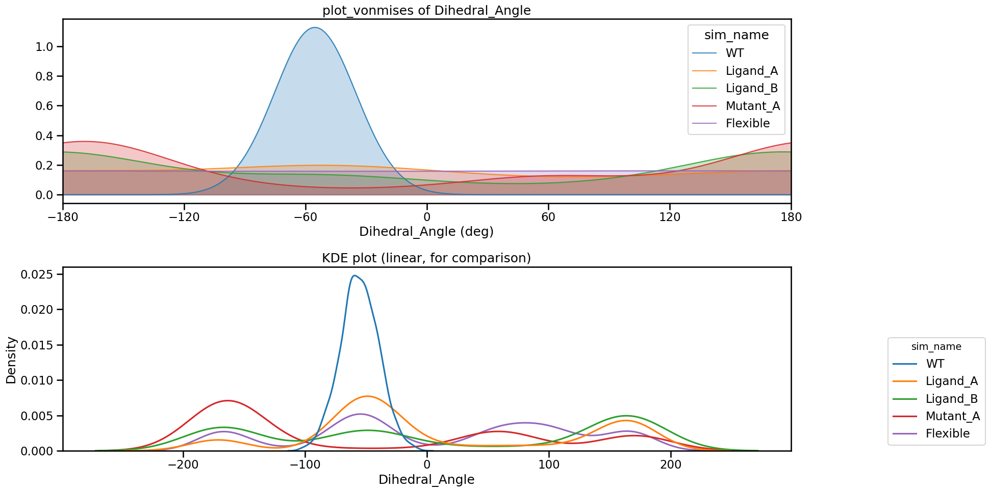
fig, axes = plt.subplots(2, 1, figsize=(20, 10))

dataset.plot_vonmises(x="Dihedral_Angle", mode="per_sim", fill=True, kappa_adjust=1.5, ax=axes[0])
dataset.plot_distri_norm(x="Dihedral_Angle", mode="per_sim", fill=False, hist=False, ax=axes[1])

axes[0].set_title("plot_vonmises of Dihedral_Angle")
axes[1].set_title("KDE plot (linear, for comparison)")

plt.tight_layout()
plt.show()
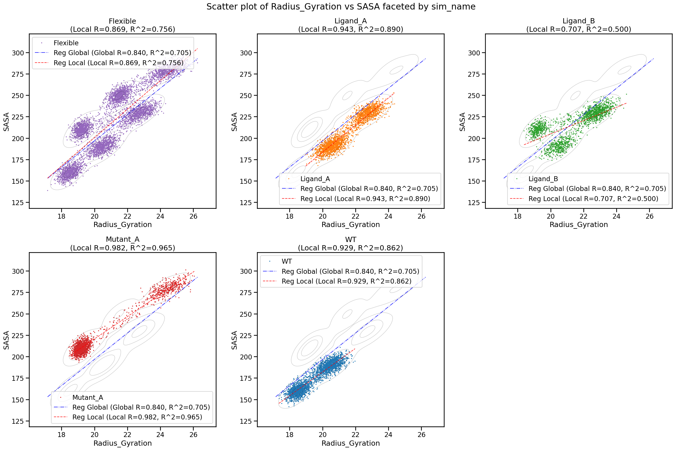
5.5 Scatter plots — plot_scatter / plot_scatter_facet
[29]:
fig, axes = dataset.plot_scatter_facet(
    x="Radius_Gyration", y="SASA", facet_col="sim_name", ncols=3, s=6, alpha=1,
    global_density=True, show_corr=True, show_local_reg=True, show_global_reg=True,
)
5.6 Cluster timelines — plot_cluster_timeline
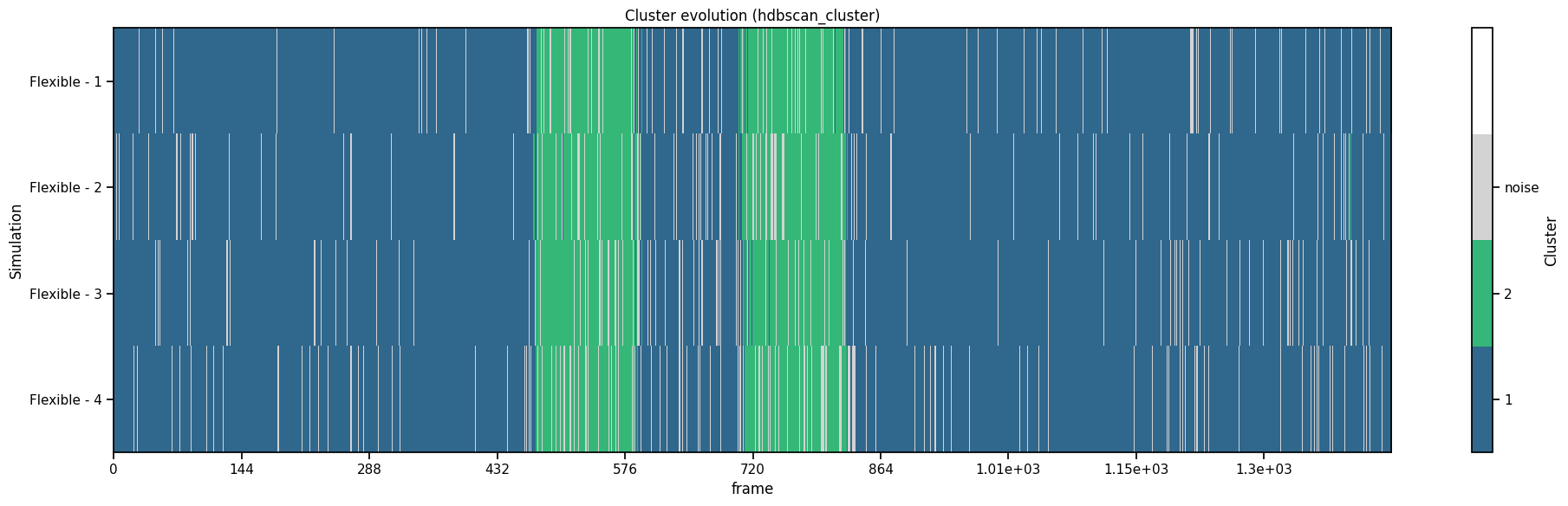
[30]:
ax, transitions = dataset.plot_cluster_timeline(
    cluster_col="hdbscan_cluster", sim_name="Flexible", time_col="frame",
    return_transitions=True, figsize=(20, 6),
)
transitions
[30]:
| sim_name | replica | n_frames | n_transitions | transition_rate | n_clusters_visited | noise_frac | dominant_cluster | dominant_frac | |
|---|---|---|---|---|---|---|---|---|---|
| 0 | Flexible | 1 | 1440 | 178 | 0.123697 | 2 | 0.061111 | 1 | 0.800000 |
| 1 | Flexible | 2 | 1440 | 178 | 0.123697 | 2 | 0.069444 | 1 | 0.791667 |
| 2 | Flexible | 3 | 1440 | 189 | 0.131341 | 2 | 0.067361 | 1 | 0.793750 |
| 3 | Flexible | 4 | 1440 | 230 | 0.159833 | 2 | 0.088889 | 1 | 0.780556 |
[31]:
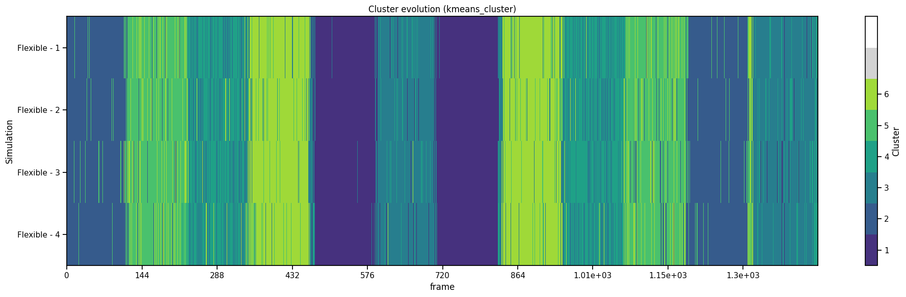
ax, transitions = dataset.plot_cluster_timeline(
    cluster_col="kmeans_cluster", sim_name="Flexible", time_col="frame",
    return_transitions=True, figsize=(20, 6),
)
transitions
[31]:
| sim_name | replica | n_frames | n_transitions | transition_rate | n_clusters_visited | noise_frac | dominant_cluster | dominant_frac | |
|---|---|---|---|---|---|---|---|---|---|
| 0 | Flexible | 1 | 1440 | 355 | 0.246699 | 6 | 0.0 | 3 | 0.216667 |
| 1 | Flexible | 2 | 1440 | 348 | 0.241835 | 6 | 0.0 | 3 | 0.220833 |
| 2 | Flexible | 3 | 1440 | 334 | 0.232106 | 6 | 0.0 | 3 | 0.213194 |
| 3 | Flexible | 4 | 1440 | 371 | 0.257818 | 6 | 0.0 | 3 | 0.218056 |
[32]:
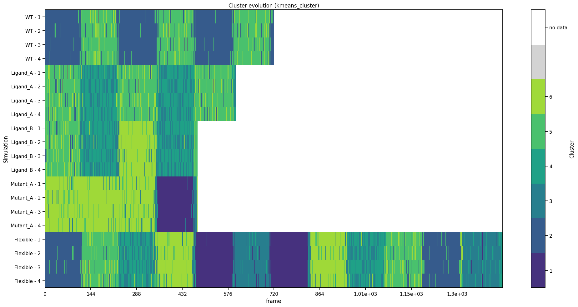
ax, transitions = dataset.plot_cluster_timeline(
    cluster_col="kmeans_cluster", time_col="frame",
    return_transitions=True, figsize=(20, 10),
)
Next steps
This covered the core workflow end to end. For the full parameter reference of every function used here (and a few more), see the per-module pages in the User Guide: Plotting, Clustering, Dimensionality reduction, and Ensemble comparison.